Sound Classification using Deep Learning

I recently completed Udacity’s Machine Learning Engineer Nanodegree Capstone Project, titled “Classifying Urban Sounds using Deep learning”, where I demonstrate how to classify different sounds using AI.
The following is an overview of the project, outlining the approach, dataset and tools used and also the results. Full links to all the code, Jupyter notebooks, and report will be posted below.
Note: I recommend running the full Jupyter notebooks in the GitHub repo rather than copy and pasting the code examples in the blog as they are not complete.
For anyone considering a taking the Udacity Machine Learning Engineer Nanodegree, I thoroughly recommend it, full course details see here.
Background
Automatic environmental sound classification is a growing area of research with numerous real world applications. Whilst there is a large body of research in related audio fields such as speech and music, work on the classification of environmental sounds is comparatively scarce.
Likewise, observing the recent advancements in the field of image classification where convolutional neural networks are used to to classify images with high accuracy and at scale, it begs the question of the applicability of these techniques in other domains, such as sound classification.
There is a plethora of real world applications for this research, such as:
• Content-based multimedia indexing and retrieval
• Assisting deaf individuals in their daily activities
• Smart home use cases such as 360-degree safety and security capabilities
• Industrial uses such as predictive maintenance
Problem statement
The following will demonstrate how to apply Deep Learning techniques to the classification of environmental sounds, specifically focusing on the identification of particular urban sounds.
When given an audio sample in a computer readable format (such as a .wav file) of a few seconds duration, we want to be able to determine if it contains one of the target urban sounds with a corresponding Classification Accuracy score.
Dataset
For this we will use a dataset called Urbansound8K. The dataset contains 8732 sound excerpts (<=4s) of urban sounds from 10 classes, which are:
• Air Conditioner
• Car Horn
• Children Playing
• Dog bark
• Drilling
• Engine Idling
• Gun Shot
• Jackhammer
• Siren
• Street Music
A sample of this dataset is included with the accompanying git repo and the full dataset can be downloaded from here.
Audio file overview
These sound excerpts are digital audio files in .wav format. Sound waves are digitised by sampling them at discrete intervals known as the sampling rate (typically 44.1kHz for CD quality audio meaning samples are taken 44,100 times per second).
Each sample is the amplitude of the wave at a particular time interval, where the bit depth determines how detailed the sample will be also known as the dynamic range of the signal (typically 16bit which means a sample can range from 65,536 amplitude values).

The above image shows how a sound excerpt is taken from a waveform and turned into a one dimensional array or vector of amplitude values.
The following is a great Youtube video for explaining the fundamental concepts of digital audio sampling.
Data Exploratory
From a visual inspection we can see that it is tricky to visualise the difference between some of the classes. Particularly, the waveforms for repetitive sounds for air conditioner, drilling, engine idling and jackhammer are similar in shape.

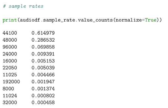
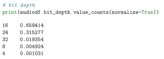
Next, we will do a deeper dive into each of the audio files properties extracting, number of audio channels, sample rate and bit-depth using the following code.
Here we can see that the dataset has a range of varying audio properties that will need standardising before we can use it to train our model.
Audio channels most of the samples have two audio channels (meaning stereo) with a few with just the one channel (mono).

Sample rate there is a wide range of Sample rates that have been used across all the samples which is a concern (ranging from 96kHz to 8kHz).

Bit-depth there is also a range of bit-depths (ranging from 4bit to 32bit).

Data pre-processing
In the previous section we identified the following audio properties that need preprocessing to ensure consistency across the whole dataset:
• Audio Channels
• Sample rate
• Bit-depth
Librosa is a Python package for music and audio processing by Brian McFee and will allow us to load audio in our notebook as a numpy array for analysis and manipulation.
For much of the preprocessing we will be able to use Librosa’s load() function, which by default converts the sampling rate to 22.05 KHz, normalise the data so the bit-depth values range between -1 and 1 and flattens the audio channels into mono.
Extract features
The next step is to extract the features we will need to train our model. To do this, we are going to create a visual representation of each of the audio samples which will allow us to identify features for classification, using the same techniques used to classify images with high accuracy.
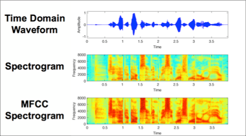
Spectrograms are a useful technique for visualising the spectrum of frequencies of a sound and how they vary during a very short period of time. We will be using a similar technique known as Mel-Frequency Cepstral Coefficients (MFCC).
The main difference is that a spectrogram uses a linear spaced frequency scale (so each frequency bin is spaced an equal number of Hertz apart), whereas an MFCC uses a quasi-logarithmic spaced frequency scale, which is more similar to how the human auditory system processes sounds.
The image below compares three different visual representations of a sound wave, the first being the time domain representation, comparing amplitude over time. The next is a spectrogram showing the energy in different frequency bands changing over time, then finally an MFCC which we can see is very similar to a spectrogram but with more distinguishable detail.

For each audio file in the dataset, we will extract an MFCC (meaning we have an image representation for each audio sample) and store it in a Panda Dataframe along with it’s classification label. For this we will use Librosa’s mfcc() function which generates an MFCC from time series audio data.
Converting the data and labels then splitting the dataset
We will use sklearn.preprocessing.LabelEncoder to encode the categorical text data into model-understandable numerical data.
Then we will use sklearn.model_selection.train_test_split to split the dataset into training and testing sets. The testing set size will be 20% and we will set a random state.
Building our model
The next step will be to build and train a Deep Neural Network with these data sets and make predictions.
Here we will use a Convolutional Neural Network (CNN). CNN’s typically make good classifiers and perform particular well with image classification tasks due to their feature extraction and classification parts. I believe that this will be very effective at finding patterns within the MFCC’s much like they are effective at finding patterns within images.
We will use a sequential model, starting with a simple model architecture, consisting of four Conv2D convolution layers, with our final output layer being a dense layer. Our output layer will have 10 nodes (num_labels) which matches the number of possible classifications.
See the full report for an in-depth breakdown of the chosen layers, we also compare the performance of the CNN with a more traditional MLP.
For compiling our model, we will use the following three parameters:
Here we will train the model. As training a CNN can take a significant amount of time, we will start with a low number of epochs and a low batch size. If we can see from the output that the model is converging, we will increase both numbers.
The following will review the accuracy of the model on both the training and test data sets.
Results
Our trained model obtained a Training accuracy of 98.19% and a Testing accuracy of 91.92%.
The performance is very good and the model has generalised well, seeming to predict well when tested against new audio data.
Observations
It was earlier noted in our data exploration, that it is difficult to visualise the difference between some of the classes. In particular, the following sub-groups are similar in shape:
• Repetitive sounds for air conditioner, drilling, engine idling and jackhammer.
• Sharp peaks for dog barking and gun shot.
• Similar pattern for children playing and street music.
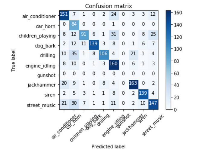
Using a confusion matrix we will examine if the final model also struggled to differentiate between these classes.

The Confusion Matrix tells a different story. Here we can see that our model struggles the most with the following sub-groups:
• air conditioner, jackhammer and street music.
• car horn, drilling, and street music.
• air conditioner, children playing and engine idling.
• jackhammer and drilling.
• air conditioner, car horn, children playing and street music.
This shows us that the problem is more nuanced than our initial assessment and gives some in- sights into the features that the CNN is extracting to make its classifications. For example, street music is one of the commonly misclassified classes and could be to a wide variety of different samples within the class.
Next steps
The next logical step is to see how the above can be applied both to Real-time streaming audio and using real world sounds.
Audio in the real world is much more of a ‘messier’ challenge, as we will need to accommodate for different background sounds, different volume levels of the target sound and the likelihood of echos.
Doing this in Real-time also poses its challenges as the model will have to perform well with low-latency, as will the MFCC calculation, all whilst synchronising with the audio buffer thread without any delays.
**I would like to write a follow up post on this if I can find the time, but will need a volunteer(s) to help, if this is something you are interested with getting involved with then do get in touch.**
Finally
Thank you for reading and if you enjoyed reading Sound Classification using Deep Learning I would encourage you to read the full report (link below). If you found this article useful, do get in touch.
I offer consultancy and pro-bono advice to startups and scaleups. You can find out more about me and contact me here mikesmales.com
If this article helped you, then please buy me a coffee (via KoFi) ☕️😀
If you want to take the Udacity Machine Learning Engineer Nanodegree (which I thoroughly recommend) full course details can be found here.
Full links to all the code, Jupyter notebooks, and report can be found on my GitHub page here:
